System of linear equations

In mathematics, a system of linear equations (or linear system) is a collection of linear equations involving the same set of variables. For example,

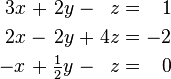
$\begin{alignat}{7} 3x &&\; + \;&& 2y &&\; - \;&& z &&\; = \;&& 1 & \\ 2x &&\; - \;&& 2y &&\; + \;&& 4z &&\; = \;&& -2 & \\ -x &&\; + \;&& \tfrac{1}{2} y &&\; - \;&& z &&\; = \;&& 0 & \end{alignat}$

is a system of three equations in the three variables $x, y, z\,\!$ . A solution to a linear system is an assignment of numbers to the variables such that all the equations are simultaneously satisfied. A solution to the system above is given by

$\begin{alignat}{2} x & = & 1 \\ y & = & -2 \\ z & = & -2 \end{alignat}$

since it makes all three equations valid.

In mathematics, the theory of linear systems is a branch of linear algebra, a subject which is fundamental to modern mathematics. Computational algorithms for finding the solutions are an important part of numerical linear algebra, and such methods play a prominent role in engineering, physics, chemistry, computer science, and economics. A system of non-linear equations can often be approximated by a linear system (see linearization), a helpful technique when making a mathematical model or computer simulation of a relatively complex system.

The simplest kind of linear system involves two equations and two variables:

$\begin{alignat}{5} 2x &&\; + \;&& 3y &&\; = \;&& 6 & \\ 4x &&\; + \;&& 9y &&\; = \;&& 15. \end{alignat}$

One method for solving such a system is as follows. First, solve the top equation for x in terms of y:

$x = 3 - \frac{3}{2}y.$

Now substitute this expression for x into the bottom equation:

$4\left( 3 - \frac{3}{2}y \right) + 9y = 15.$

This results in a single equation involving only the variable y. Solving gives y = 1, and substituting this back into the equation for x yields x = 3/2.

General form

A general system of m linear equations with n unknowns can be written as

$\begin{alignat}{7} a_{11} x_1 &&\; + \;&& a_{12} x_2 &&\; + \cdots + \;&& a_{1n} x_n &&\; = \;&&& b_1 \\ a_{21} x_1 &&\; + \;&& a_{22} x_2 &&\; + \cdots + \;&& a_{2n} x_n &&\; = \;&&& b_2 \\ \vdots\;\;\; && && \vdots\;\;\; && && \vdots\;\;\; && &&& \;\vdots \\ a_{m1} x_1 &&\; + \;&& a_{m2} x_2 &&\; + \cdots + \;&& a_{mn} x_n &&\; = \;&&& b_m. \\ \end{alignat}$

Here $x_1,\ x_2,...,x_n$ are the unknowns, $a_{11},\ a_{12},...,\ a_{mn}$ are the coefficients of the system, and $b_1,\ b_2,...,b_m$ are the constant terms.

Vector equation

One extremely helpful view is that each unknown is a weight for a column vector in a linear combination.

$x_1 \begin{bmatrix}a_{11}\\a_{21}\\ \vdots \\a_{m1}\end{bmatrix} + x_2 \begin{bmatrix}a_{12}\\a_{22}\\ \vdots \\a_{m2}\end{bmatrix} + \cdots + x_n \begin{bmatrix}a_{1n}\\a_{2n}\\ \vdots \\a_{mn}\end{bmatrix} = \begin{bmatrix}b_1\\b_2\\ \vdots \\b_m\end{bmatrix}$

Matrix equation

The vector equation is equivalent to a matrix equation of the form

$A\bold{x}=\bold{b}$

where A is an m×n matrix, x is a column vector with n entries, and b is a column vector with m entries.

$A= \begin{bmatrix} a_{11} & a_{12} & \cdots & a_{1n} \\ a_{21} & a_{22} & \cdots & a_{2n} \\ \vdots & \vdots & \ddots & \vdots \\ a_{m1} & a_{m2} & \cdots & a_{mn} \end{bmatrix},\quad \bold{x}= \begin{bmatrix} x_1 \\ x_2 \\ \vdots \\ x_n \end{bmatrix},\quad \bold{b}= \begin{bmatrix} b_1 \\ b_2 \\ \vdots \\ b_m \end{bmatrix}$

The number of vectors in a basis for the span is now expressed as the rank of the matrix.

Solution set

A solution of a linear system is an assignment of values to the variables x₁, x₂, ..., x_n such that each of the equations is satisfied. The set of all possible solutions is called the solution set.

A linear system may behave in any one of three possible ways:

The system has infinitely many solutions.
The system has a single unique solution.
The system has no solutions.

Geometric interpretation

The solution set for the equations x – y = –1 and 3x + y = 9 is the single point (2, 3).

For a system involving two variables (x and y), each linear equation determines a line on the xy-plane. Because a solution to a linear system must satisfy all of the equations, the solution set is the intersection of these lines, and is hence either a line, a single point, or the empty set.

For three variables, each linear equation determines a plane in three-dimensional space, and the solution set is the intersection of these planes. Thus the solution set may be a plane, a line, a single point, or the empty set.

For n variables, each linear equations determines a hyperplane in n-dimensional space. The solution set is the intersection of these hyperplanes, which may be a flat of any dimension.

General behavior

The solution set for two equations in three variables is usually a line.

In general, the behavior of a linear system is determined by the relationship between the number of equations and the number of unknowns:

Usually, a system with fewer equations than unknowns has infinitely many solutions.
Usually, a system with the same number of equations and unknowns has a single unique solution.
Usually, a system with more equations than unknowns has no solution.

In the first case, the dimension of the solution set is usually equal to n – m, where n is the number of variables and m is the number of equations.

The following pictures illustrate this trichotomy in the case of two variables:


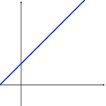
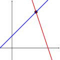
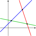
One Equation	Two Equations	Three Equations

The first system has infinitely many solutions, namely all of the points on the blue line. The second system has a single unique solution, namely the intersection of the two lines. The third system has no solutions, since the three lines share no common point.

Keep in mind that the pictures above show only the most common case. It is possible for a system of two equations and two unknowns to have no solution (if the two lines are parallel), or for a system of three equations and two unknowns to be solvable (if the three lines intersect at a single point). In general, a system of linear equations may behave differently than expected if the equations are linearly dependent, or if two or more of the equations are inconsistent.

Properties

Consistency

The equations 3x + 2y = 6 and 3x + 2y = 12 are inconsistent.

The equations of a linear system are consistent if they possess a common solution, and inconsistent otherwise. When the equations are inconsistent, it is possible to derive a contradiction from the equations, such as the statement that 0 = 1.

For example, the equations

$3x+2y=6\;\;\;\;\text{and}\;\;\;\;3x+2y=12$

are inconsistent. In attempting to find a solution, we tacitly assume that there is a solution; that is, we assume that the value of x in the first equation must be the same as the value of x in the second equation (the same is assumed to simultaneously be true for the value of y in both equations). Applying the substitution property (for 3x+2y) yields the equation 6 = 12, which is a false statement. This therefore contradicts our assumption that the system had a solution and we conclude that our assumption was false; that is, the system in fact has no solution. The graphs of these equations on the xy-plane are a pair of parallel lines.

It is possible for three linear equations to be inconsistent, even though any two of the equations are consistent together. For example, the equations

$\begin{alignat}{7} x &&\; + \;&& y &&\; = \;&& 1 & \\ 2x &&\; + \;&& y &&\; = \;&& 1 & \\ 3x &&\; + \;&& 2y &&\; = \;&& 3 & \end{alignat}$

are inconsistent. Adding the first two equations together gives 3x + 2y = 2, which can be subtracted from the third equation to yield 0 = 1. Note that any two of these equations have a common solution. The same phenomenon can occur for any number of equations.

In general, inconsistencies occur if the left-hand sides of the equations in a system are linearly dependent, and the constant terms do not satisfy the dependence relation. A system of equations whose left-hand sides are linearly independent is always consistent.

Independence

The equations of a linear system are independent if none of the equations can be derived algebraically from the others. When the equations are independent, each equation contains new information about the variables, and removing any of the equations increases the size of the solution set. For linear equations, logical independence is the same as linear independence.

The equations x – 2y = –1, 3x + 5y = 8, and 4x + 3y = 7 are not linearly independent.

For example, the equations

$3x+2y=6\;\;\;\;\text{and}\;\;\;\;6x+4y=12$

are not independent. The second equation is just the first equation multiplied by two (and the first equation is the second equation divided by two). The graphs of these two equations are the same.

For a more complicated example, the equations

$\begin{alignat}{5} x &&\; - \;&& 2y &&\; = \;&& -1 & \\ 3x &&\; + \;&& 5y &&\; = \;&& 8 & \\ 4x &&\; + \;&& 3y &&\; = \;&& 7 & \end{alignat}$

are not independent, because the third equation is the sum of the other two. Indeed, any one of these equations can be derived from the other two, and any one of the equations can be removed without affecting the solution set. The graphs of these equations are three lines that intersect at a single point.

Equivalence

Two linear systems using the same set of variables are equivalent if each of the equations in the second system can be derived algebraically from the equations in the first system, and vice-versa. Equivalent systems convey precisely the same information about the values of the variables. In particular, two linear systems are equivalent if and only if they have the same solution set.

Solving a linear system

There are several algorithms for solving a system of linear equations.

Describing the solution

It can be difficult to describe the solution set to a linear system with infinitely many solutions. Typically, some of the variables are designated as free (or independent, or as parameters), meaning that they are allowed to take any value, while the remaining variables are dependent on the values of the free variables.

For example, consider the following system:

$\begin{alignat}{7} x &&\; + \;&& 3y &&\; - \;&& 2z &&\; = \;&& 5 & \\ 3x &&\; + \;&& 5y &&\; + \;&& 6z &&\; = \;&& 7 & \end{alignat}$

The solution set to this system can be described by the following equations:

$x=-7z-1\;\;\;\;\text{and}\;\;\;\;y=3z+2\text{.}$

Here z is the free variable, while x and y are dependent on z. Any point in the solution set can be obtained by first choosing a value for z, and then computing the corresponding values for x and y.

Each free variable gives the solution space one degree of freedom, the number of which is equal to the dimension of the solution set. For example, the solution set for the above equation is a line, since a point in the solution set can be chosen by specifying the value of the parameter z.

Different choices for the free variables may lead to different descriptions of the same solution set. For example, the solution to the above equations can alternatively be described as follows:

$y=-\frac{3}{7}x + \frac{11}{7}\;\;\;\;\text{and}\;\;\;\;z=-\frac{1}{7}x-\frac{1}{7}\text{.}$

Here x is the free variable, and y and z are dependent.

Elimination of variables

The simplest method for solving a system of linear equations is to repeatedly eliminate variables. This method can be described as follows:

In the first equation, solve for the one of the variables in terms of the others.
Plug this expression into the remaining equations. This yields a system of equations with one fewer equation and one fewer unknown.
Continue until you have reduced the system to a single linear equation.
Solve this equation, and then back-substitute until the entire solution is found.

For example, consider the following system:

$\begin{alignat}{7} x &&\; + \;&& 3y &&\; - \;&& 2z &&\; = \;&& 5 & \\ 3x &&\; + \;&& 5y &&\; + \;&& 6z &&\; = \;&& 7 & \\ 2x &&\; + \;&& 4y &&\; + \;&& 3z &&\; = \;&& 8 & \end{alignat}$

Solving the first equation for x gives x = 5 + 2z – 3y, and plugging this into the second and third equation yields

$\begin{alignat}{5} -4y &&\; + \;&& 12z &&\; = \;&& -8 & \\ -2y &&\; + \;&& 7z &&\; = \;&& -2 & \end{alignat}$

Solving the first of these equations for y yields y = 2 + 3z, and plugging this into the third equation yields z = 2. We now have:

$\begin{alignat}{7} x &&\; = \;&& 5 &&\; + \;&& 2z &&\; - \;&& 3y & \\ y &&\; = \;&& 2 &&\; + \;&& 3z && && & \\ z &&\; = \;&& 2 && && && && & \end{alignat}$

Substituting z = 2 into the second equation gives y = 8, and substituting z = 2 and y = 8 into the first equation yields x = –15. Therefore, the solution set is the single point (x, y, z) = (–15, 8, 2).

Row reduction

Main article: Gaussian elimination

In row reduction, the linear system is represented as an augmented matrix:

$\left[\begin{array}{rrr|r} 1 & 3 & -2 & 5 \\ 3 & 5 & 6 & 7 \\ 2 & 4 & 3 & 8 \end{array}\right]\text{.}$

This matrix is then modified using elementary row operations until it reaches reduced row echelon form. There are three types of elementary row operations:

Type 1: Swap the positions of two rows.

Type 2: Multiply a row by a nonzero scalar.

Type 3: Add to one row a scalar multiple of another.

Because these operations are reversible, the augmented matrix produced always represents a linear system that is equivalent to the original.

There are several specific algorithms to row-reduce an augmented matrix, the simplest of which are Gaussian elimination and Gauss-Jordan elimination. The following computation shows Gaussian elimination applied to the matrix above:

$\left[\begin{array}{rrr|r} 1 & 3 & -2 & 5 \\ 3 & 5 & 6 & 7 \\ 2 & 4 & 3 & 8 \end{array}\right]$ $\sim \left[\begin{array}{rrr|r} 1 & 3 & -2 & 5 \\ 0 & -4 & 12 & -8 \\ 2 & 4 & 3 & 8 \end{array}\right]$ $\sim \left[\begin{array}{rrr|r} 1 & 3 & -2 & 5 \\ 0 & -4 & 12 & -8 \\ 0 & -2 & 7 & -2 \end{array}\right]$ $\sim \left[\begin{array}{rrr|r} 1 & 3 & -2 & 5 \\ 0 & 1 & -3 & 2 \\ 0 & -2 & 7 & -2 \end{array}\right]$ $\sim \left[\begin{array}{rrr|r} 1 & 3 & -2 & 5 \\ 0 & 1 & -3 & 2 \\ 0 & 0 & 1 & 2 \end{array}\right]$ $\sim \left[\begin{array}{rrr|r} 1 & 3 & -2 & 5 \\ 0 & 1 & 0 & 8 \\ 0 & 0 & 1 & 2 \end{array}\right]$ $\sim \left[\begin{array}{rrr|r} 1 & 3 & 0 & 9 \\ 0 & 1 & 0 & 8 \\ 0 & 0 & 1 & 2 \end{array}\right]$ $\sim \left[\begin{array}{rrr|r} 1 & 0 & 0 & -15 \\ 0 & 1 & 0 & 8 \\ 0 & 0 & 1 & 2 \end{array}\right].$

The last matrix is in reduced row echelon form, and represents the system x = –15, y = 8, z = 2. A comparison with the example in the previous section on the algebraic elimination of variables shows that these two methods are in fact the same; the difference lies in how the

Cramer's rule

Main article: Cramer's rule

Cramer's rule is an explicit formula for the solution of a system of linear equations, with each variable given by a quotient of two determinants. For example, the solution to the system

$\begin{alignat}{7} x &&\; + \;&& 3y &&\; - \;&& 2z &&\; = \;&& 5 & \\ 3x &&\; + \;&& 5y &&\; + \;&& 6z &&\; = \;&& 7 & \\ 2x &&\; + \;&& 4y &&\; + \;&& 3z &&\; = \;&& 8 & \end{alignat}$

is given by

$x=\frac {\,\left| \begin{matrix}5&3&-2\\7&5&6\\8&4&3\end{matrix} \right|\,} {\,\left| \begin{matrix}1&3&-2\\3&5&6\\2&4&3\end{matrix} \right|\,} ,\;\;\;\;y=\frac {\,\left| \begin{matrix}1&5&-2\\3&7&6\\2&8&3\end{matrix} \right|\,} {\,\left| \begin{matrix}1&3&-2\\3&5&6\\2&4&3\end{matrix} \right|\,} ,\;\;\;\;z=\frac {\,\left| \begin{matrix}1&3&5\\3&5&7\\2&4&8\end{matrix} \right|\,} {\,\left| \begin{matrix}1&3&-2\\3&5&6\\2&4&3\end{matrix} \right|\,}.$

For each variable, the denominator is the determinant of the matrix of coefficients, while the numerator is the determinant of a matrix in which one column has been replaced by the vector of constant terms.

Though Cramer's rule is important theoretically, it has little practical value for large matrices, since the computation of large determinants is somewhat cumbersome. (Indeed, large determinants are most easily computed using row reduction.) Further, Cramer's rule has very poor numerical properties, making it unsuitable for solving even small systems reliably, unless the operations are performed in rational arithmetic with unbounded precision.

THE END>>>>>>>>>>>^_^

GiLoNiTy

Sunday, January 11, 2009